Convolution Layers¶

Overview
Implementation
Examples
API

Overview ¶

DistDL’s The Distributed Convolutional layers use the distributed primitive layers to build various distributed versions of PyTorch ConvXd layers. That is, it implements

\[y = w*x + b\]

where \(*\) is the convolution operator and the tensors \(x\), \(y\), \(w\), and \(b\) are partitioned over a number of workers.

For the purposes of this documentation, we will assume that an arbitrary global input tensor \({x}\) is partitioned by \(P_x\). Another partition \(P_y\), may exist depending on implementation. similarly, the weight tensor \(w\) may also have its own partition is partitioned by \(P_w\). The bias \(b\) is implicitly partitioned depending on the nature of \(P_w\).

Implementation ¶

The partitioning of the input and output tensors strongly impacts the necessary operations to perform a distributed convolution. Consequently, DistDL has multiple implementations to satisfy some special cases and the general case.

Public Interface ¶

DistDL provides a public interface to the many distributed convolution implementations that follows the same pattern as other public interfaces, such as the Linear Layer and keeping in line with the PyTorch interface. The distdl.nn.conv module provides the distdl.nn.conv.DistributedConv1d, distdl.nn.conv.DistributedConv2d, and distdl.nn.conv.DistributedConv3d types, which through use the class distdl.nn.conv.DistributedConvSelector to dispatch an appropriate implementation, based on the structure of \(P_x\), \(P_y\), and \(P_W\).

Current implementations include those for:

Feature-distributed Convolution
Channel-distributed Convolution
Generalized Distributed Convolution

Feature-distributed Convolution ¶

The simplest distributed convolution implementation, and the one that generally requires the least workers, has input (and outout) tensors that are distributed in feature-space only. This is also, likely, the most common use-case.

Construction of this layer is driven by the partitioning of the input tensor \(x\), only. Thus, the partition \(P_x\) drives the algorithm design. With a pure feature-space partition, the output partition will have the same structure, so there is no need to specify it. Also, with no partition in the channel dimension, the learnable weight tensor is assumed to be small enough that it can trivially be stored by one worker.

Assumptions¶

The global input tensor \(x\) has shape \(n_{\text{b}} \times n_{c_{\text{in}}} \times n_{D-1} \times \cdots \times n_0\).
The input partition \(P_x\) has shape \(1 \times 1 \times P_{D-1} \times \cdots \times P_0\), where \(P_{d}\) is the number of workers partitioning the \(d^{\text{th}}\) feature dimension of \(x\).
The global output tensor \(y\) will have shape \(n_{\text{b}} \times n_{c_{\text{out}}} \times m_{D-1} \times \cdots \times m_0\). The precise values of \(m_{D-1} \times \cdots \times m_0\) are dependent on the input shape and the kernel parameters.
The output partition \(P_y\) implicitly has the same shape as \(P_x\).
The weight tensor \(w\) will have shape \(n_{c_{\text{out}}} \times n_{c_{\text{in}}} \times k_{D-1} \times \cdots \times k_0\).
The weight partition does not necessarily explicitly exist, but implicitly has shape \(1 \times 1 \times 1 \times \cdots \times 1\).
Any learnable bias is stored on the same worker as the learnable weights.

Example setup for feature-distributed convolutional layer. — An example setup for a 1D distributed convolutional layer, where \(P_x\) has shape \(1 \times 1 \times 4\), \(P_y\) has the same shape, and \(P_W\) has shape \(1 \times 1 \times 1\).¶

Forward¶

Under the above assumptions, the forward algorithm is:

Use a Broadcast Layer to broadcast the learnable \(w\) from a single worker in \(P_x\) to all of \(P_x\). If necessary, a different broadcast layer, also from a single worker in \(P_x\) to all of \(P_x\) broadcasts the learnable bias \(b\).

The weight and bias tensors, post broadcast, are used by the local convolution.

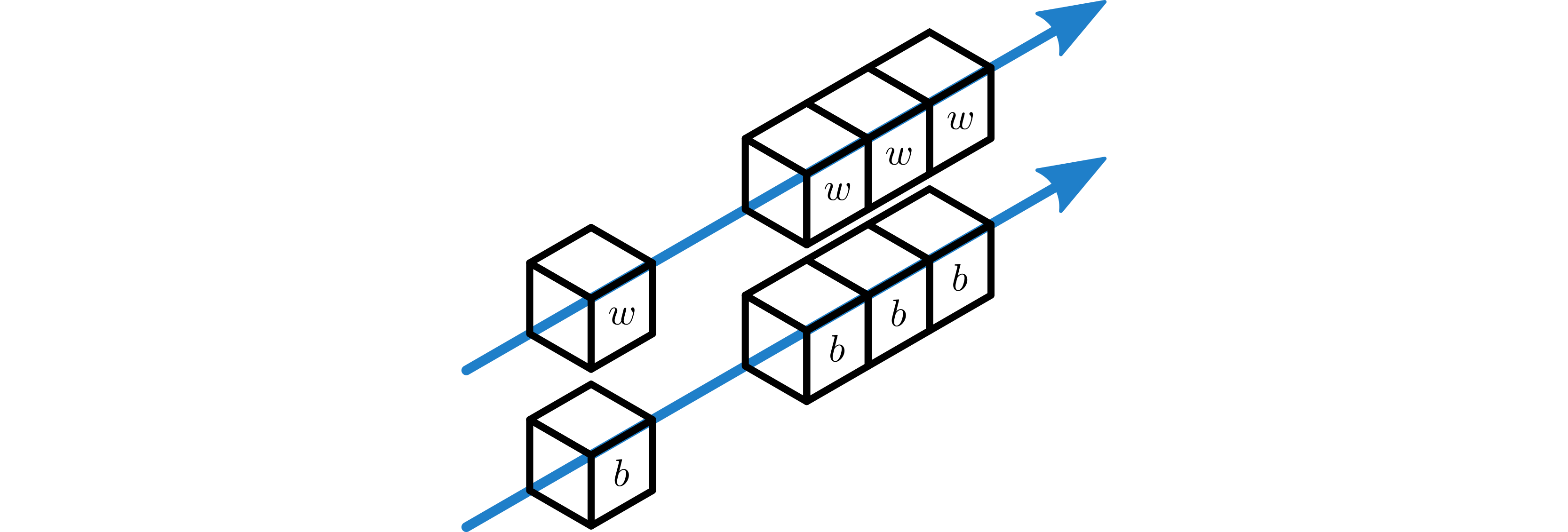
Example forward broadcast in the feature-distributed convolutional layer. — \(w\) and \(b\) are broadcast to all workers in \(P_x\).¶

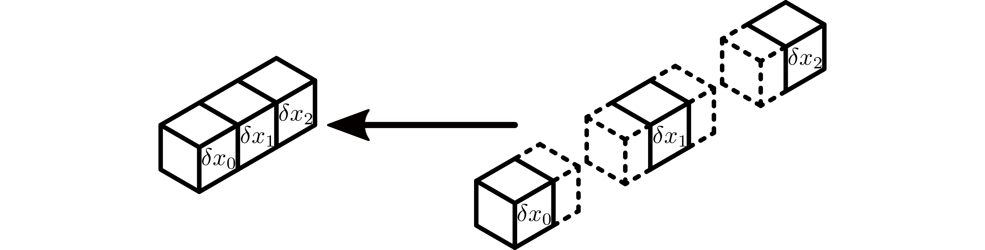
Perform the halo exchange on the subtensors of \(x\). Here, \(x_j\) must be padded to accept local halo regions (in a potentially unbalanced way) before the halos are exchanged. The output of this operation is \(\hat x_j\).

Example forward padding of subtensors of x in feature-distributed convolutional layer. — Subtensors of \(x\), \(x_j\) must be padded to accept the halo data.¶

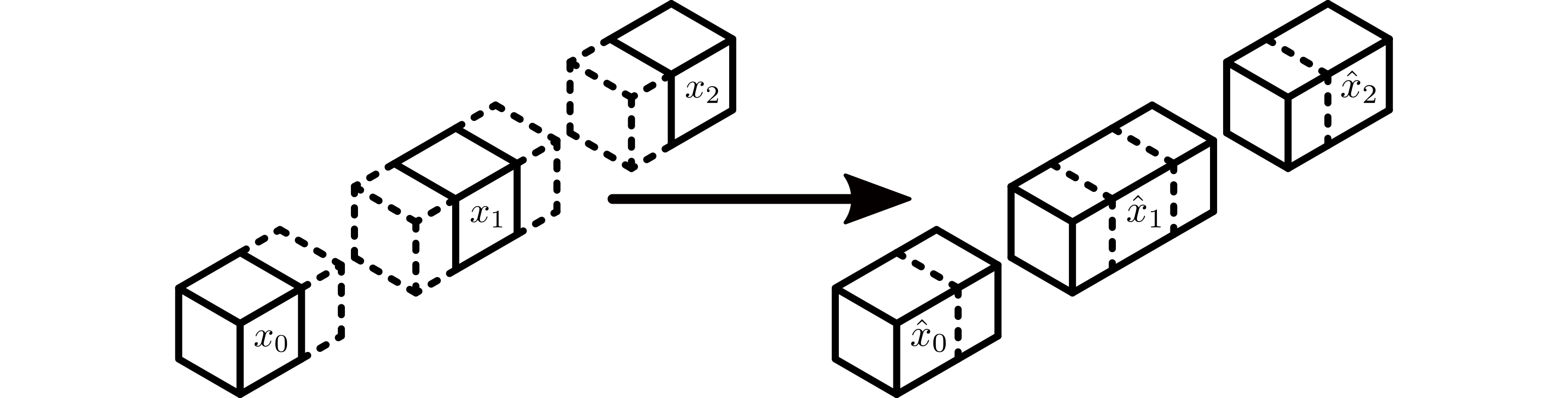
Example forward halo exchange on subtensors of x in feature-distributed convolutional layer. — Forward halos are exchanged on \(P_x\), creating \(\hat x_j\).¶

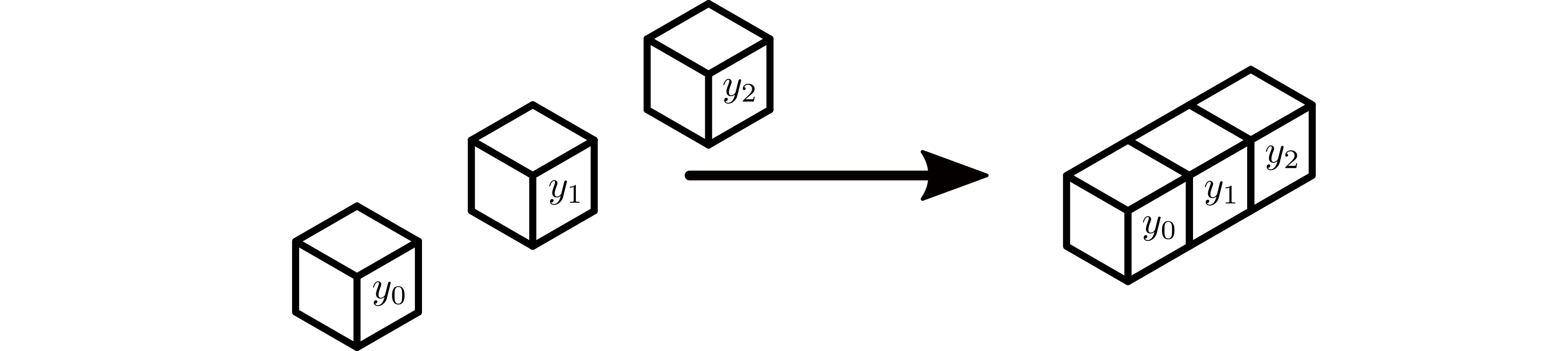
Perform the local forward convolution application using a PyTorch ConvXd layer. The bias is added everywhere, as each workers output will be part of the output tensor.

Example forward convolution in the feature-distributed convolutional layer. — The \(y_i\) subtensors are computed using native PyTorch layers.¶

The subtensors in the inputs and outputs of DistDL layers should always be able to be reconstructed into precisely the same tensor a sequential application will produce. Because padding is explicitly added to the input tensor to account for the padding specified for the convolution, the output of the local convolution, \(y_i\), should exactly match that of the sequential layer.

Example forward result of the feature-distributed convolutional layer.

Adjoint¶

The adjoint algorithm is not explicitly implemented. PyTorch’s autograd feature automatically builds the adjoint of the Jacobian of the feature-distributed convolution forward application. Essentially, the algorithm is as follows:

The gradient output \(\delta y_i\) is already distributed across its partition, so the adjoint of the Jacobian of the local convolutional layer can be applied to it.

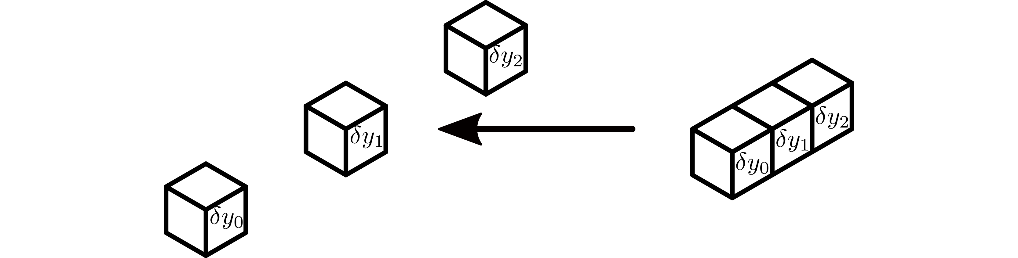
Example adjoint starting case in the feature-distributed convolutional layer.

Each worker computes its local contribution to \(\delta w\) and \(\delta x\), given by \(\delta w_j\) and \(\delta x_j\), using PyTorch’s native implementation of the adjoint of the Jacobian of the local sequential convolutional layer. If the bias is required, each worker computes its local contribution to \(\delta b_j\), \(\delta \hat b\) similarly.

Example adjoint convolution in the feature-distributed convolutional layer. — Subtensors of \(\delta w_j\), \(\delta \hat x_j\), and \(\delta b_j\) are computed using native PyTorch layers.¶

The adjoint of the halo exchange is applied to \(\delta \hat x\), which is then unpadded, producing the gradient input \(\delta x\).

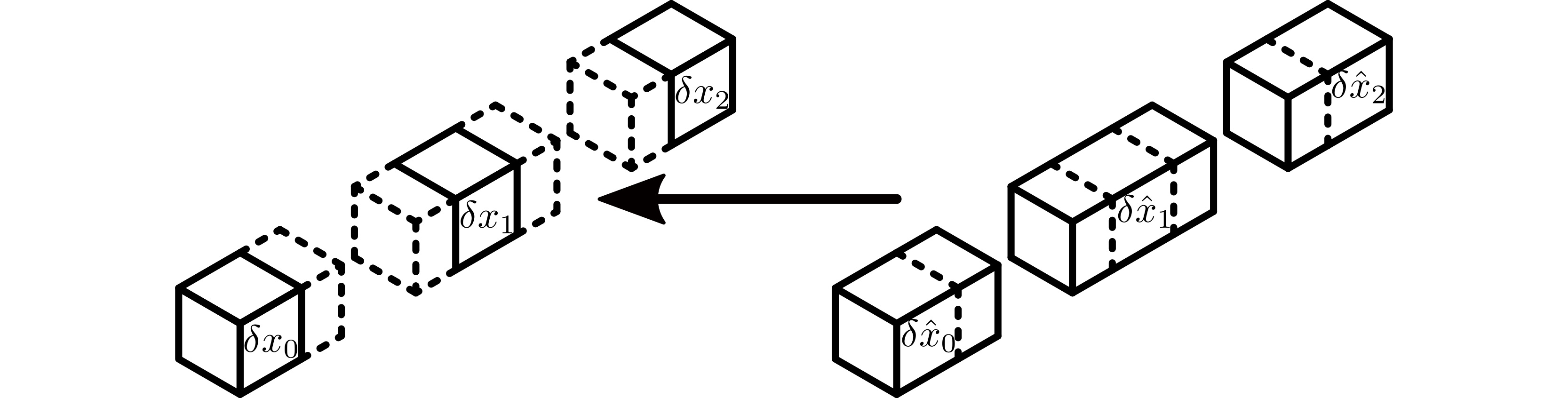
Example adjoint halo exchange on subtensors of dx in feature-distributed convolutional layer. — Adjoint halos of \(\delta \hat x\) are exchanged on the \(P_x\).¶

Example adjoint padding (unpadding) of subtensors of delta x in feature-distributed convolutional layer. — Subtensors \(\delta \hat x_j\) must be unpadded to after the halo regions are cleared :to create, creating \(\delta x\).¶

Sum-reduce the partial weight gradients, \(\delta w_j\), to produce the total gradient \(\delta w\) on the relevant worker in \(P_x\).

If required, do the same thing to produce \(\delta b\) from each worker’s \(\delta b_j\).

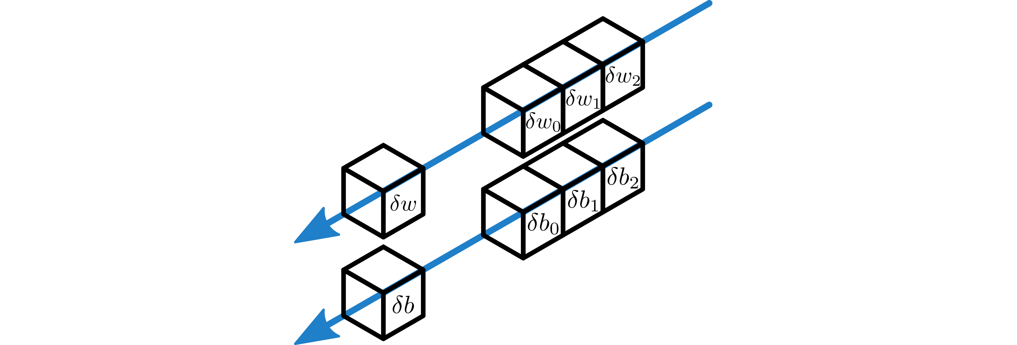
Example adjoint broadcast in the feature-distributed convolutional layer. — \(\delta w\) and \(\delta b\) are constructed from a sum-reduction on all workers in \(P_x\).¶

Channel-distributed Convolution ¶

DistDL provides a distributed convolution layer that supports partitions in the channel-dimension only. This pattern may be useful when layers are narrow in feature space.

For the construction of this layer, we assume that the fundamental unit of work is driven by dense channels in \(w\). Thus, the structure of the partition \(P_w\) drives the design. This layer admits differences between \(P_x\) and \(P_y\), so all three partitions, including \(P_w\), must be specified. It is assumed that there is no partitioning in the feature-space for the input and output tensors.