Linear Layer

Overview

The Distributed Linear (or affine) layer uses distributed primitive layers to build a distributed version of the PyTorch Linear layer. That is, it implements

\[y = Wx + b\]

where the tensors \(x\), \(y\), \(W\), and \(b\) are partitioned over a number of workers.

For the purposes of this documentation, we will assume that an arbitrary global input tensor \({x}\) is partitioned by \(P_x\) and that another partition \(P_y\) exists. Additionally, we will assume that the weight tensor \(W\) is partitioned by \(P_W\). The bias \(b\) is implicitly partitioned.

Implementation

For the construction of this layer, we assume that the fundamental unit of work is driven by dense subtensors of \(W\). Thus, the structure of the partition \(P_W\) drives the design.

The distributed linear layer is an application of distributed GEMM. The optimal implementation will be system and problem dependent. The current implementation is greedy from the perspective of the number of workers.

Note

Other algorithms, which reduce the number of required workers can be built from similar primitives. We are happy to implement those if they are suggested.

The current implementation stores the learnable weights and biases inside local sequential Linear layer functions. To avoid double counting the bias, only a subset of these local sequential Linear layers has an active bias vector.

Assumptions

• The global input tensor \(x\) has shape \(n_{\text{batch}} \times n_{\text{features in}}\).

• The input partition \(P_x\) has shape \(1 \times P_{\text{f_in}}\), where \(P_{\text{f_in}}\) is the number of workers partitioning the feature dimension of \(x\).

• The global output tensor \(y\) has shape \(n_{\text{batch}} \times n_{\text{features out}}\).

• The output partition \(P_y\) has shape \(1 \times P_{\text{f_out}}\), where \(P_{\text{f_out}}\) is the number of workers partitioning the feature dimension of \(y\).

Note

PyTorch admits input tensors of shape \(n_{\text{batch}} \times \dots \times n_{\text{features in}}\) and output tensors of shape \(n_{\text{batch}} \times \dots \times n_{\text{features out}}\). DistDL does not explicitly support intermediate dimensions at this time.

• The weight tensor \(W\) has shape \(n_{\text{features_out}} \times n_{\text{features_in}}\). This follows PyTorch.

• The weight partition \(P_W\) has shape \(P_{\text{f_out}} \times P_{\text{f_in}}\).

Note

The bias vectors are stored on the 0th column of \(P_w\). Hence, it is implicitly partitioned by a factor of \(P_{\text{f_in}}\). Following PyTorch, if the bias is turned off, no subtensors have bias terms.

An example setup for a distributed linear layer, where \(P_x\) has shape \(1 \times 4\), \(P_y\) has shape \(1 \times 3\), and \(P_W\) has shape \(3 \times 4\).

Forward

Under the above assumptions, the forward algorithm is:

1. Use a Broadcast Layer to broadcast subtensors of \(x\) from \(P_x\) over the columns of \(P_W\).

Subtensors of \(x\) are broadcast down the four columns of \(P_W\).

2. Perform the local forward linear layer application using a PyTorch Linear layer. Note that the bias is only added on the 0th column of \(P_W\). Each worker now has a portion of the output vector \(y\). In the rows of \(P_W\) the results are partial contributions to the output feature degrees-of-freedom.

Local application of linear layer. Bias is present only in 0th column.

3. Use a SumReduce Layer to reduce the subtensors of \(y\) over the rows of \(P_W\) into \(P_y\). Only one subtensor in each row of \(P_W\) contains the a subtensor of the bias, so the output tensor correctly assimilates the bias.

   Note

   This sum-reduction requires one of the partitions to be transposed.

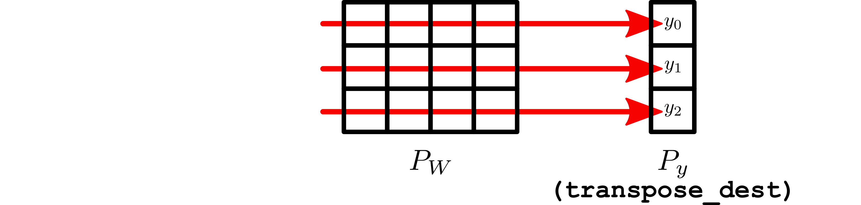
Subtensors of \(y\) are assembled via sum-reduction along the three rows of \(P_W\).

Adjoint

The adjoint algorithm is not explicitly implemented. PyTorch’s autograd feature automatically builds the adjoint of the Jacobian of the distributed linear forward application. Essentially, the algorithm is as follows:

1. Broadcast the subtensors of the gradient output, \(\delta y\) from \(P_y\) along the rows of \(P_W\).

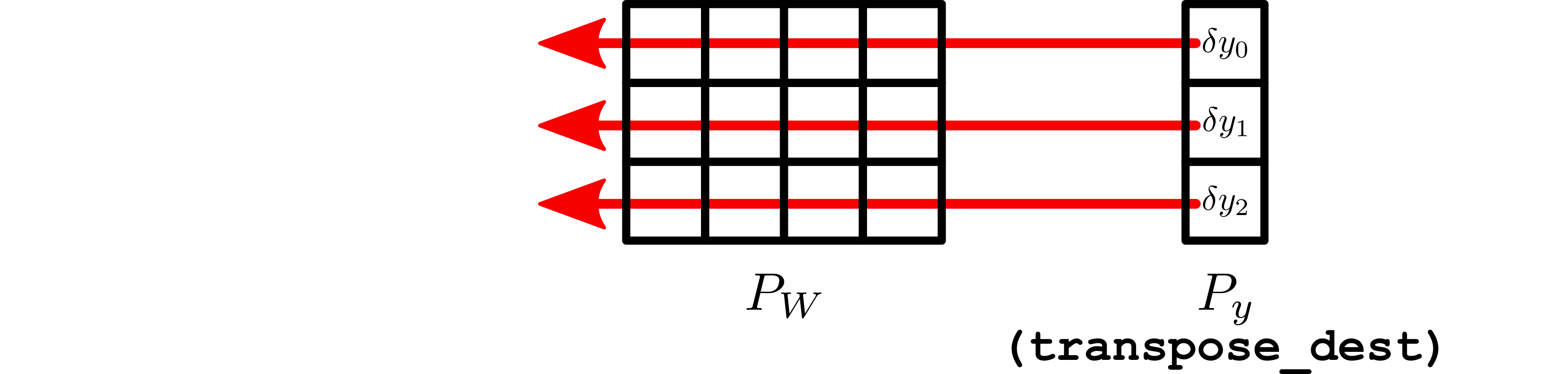
Subtensors of \(\delta y\) are broadcast across the three rows of \(P_W\).

2. Each worker in \(P_W\) computes its local part of \(\delta W\) and \(\delta x\) using the PyTorch implementation of the adjoint of the Jacobian of the local sequential linear layer. If the bias is required, the 0th column of \(P_W\) also computes \(\delta b\) similarly.

Local computation of subtensors of \(\delta x\), \(\delta W\), and \(\delta b\).

3. Sum-reduce the subtensors of the gradient input, \(\delta x\), along the rows of \(P_W\) into \(P_x\).

Subtensors of \(\delta x\) are assembled via sum-reduction along the four columns of \(P_W\).

Examples

To apply a linear layer which maps a tensor on a 1 x 4 partition to a tensor on a 1 x 3 partition:

>>> P_x_base = P_world.create_partition_inclusive(np.arange(0, 4))
>>> P_x = P_x_base.create_cartesian_topology_partition([1, 4])
>>>
>>> P_y_base = P_world.create_partition_inclusive(np.arange(4, 7))
>>> P_y = P_y_base.create_cartesian_topology_partition([1, 3])
>>>
>>> P_W_base = P_world.create_partition_inclusive(np.arange(0, 12))
>>> P_W = P_W_base.create_cartesian_topology_partition([3, 4])
>>>
>>> in_features = 16
>>> out_features = 12
>>>
>>> x_local_shape = np.array([1, 4])
>>>
>>> layer = DistributedLinear(P_x, P_y, P_W, in_features, out_features)
>>>
>>> x = zero_volume_tensor()
>>> if P_x.active:
>>>     x = torch.rand(*x_local_shape)
>>>
>>> y = layer(x)

API