distdl.backends

Overview

Data Movement Backend Interface

Each back-end will is responsible for providing the concrete definitions of partition classes and the functional interfaces for primitive data movement layers.

Partitions

Currently, two partition classes must be provided for a fully compatible back-end: Partition for partitions with no topology and CartesianPartition for partitions with a Cartesian topology.

The partition classes serve as wrappers around the back-end data movement tool’s interface. Implementations are free to make use of any back-end specific API, but in general that API should not be explicitly exposed to DistDL users.

The interfaces defined in these classes inherit a number of concepts from the MPI back-end. As DistDL evolves, it is anticipated that these interfaces can become more generalized.

Partition interfaces are explicitly for distributed communication and data movement, and as such they provide some interfaces for general parallel communication concepts (e.g., broadcasts and all-gathers) for use other than tensor data movement. While much of the interface is inspired by MPI’s API, MPI-specific terminology is avoided, e.g., we use broadcast_data, not bcast_data.

Partitions with No Topology

Back-end	Module	Class Definition	Public Alias
MPI	backends.mpi.partition	MPIPartition	Partition

The partition with no topology, exposed from each back-end as Partition, is the general container for an unstructured team of workers. It must provide interfaces for creating teams of workers, creating sub-teams of workers, creating unions of teams of workers, etc.

Regardless of back-end, a number of core partition concepts are to be exposed by a basic unstructured partition:

• size: The number of workers in the partition.

• rank: The lexicographic identifier of the current worker.

• active: The status of a worker in a partition. An active member of a partition has the ability to communicate with other workers. An inactive member has no knowledge of the other workers and is entirely disconnected from the set of active workers.

For convenience, we also allow topology-free partitions to be treated as if they are endowed with a 1-dimensional Cartesian topology. Consequently, they also have two further exposed concepts:

• shape: Always a 1-iterable with containing size as the value.

• index: Always the rank.

A partition must also provide the following API for creating new partitions:

• __init__(): A partition is initialized using whatever back-end specific information is required to determine the above properties.

• create_partition_inclusive(): Creates a subpartition of the current partition inclusive of a specified subset of workers.

• create_partition_union(): Creates a new partition containing the union of the workers in two different partitions. Workers calling instance are to be ordered before workers in the other instance and workers cannot be repeated.

• create_cartesian_topology_partition(): Using the workers in the team for the unstructured partition, create a partition endowed with a Cartesian topology.

• create_allreduction_partition(): Create the partition required to support the All-sum-reduce operation.

• create_broadcast_partition_to(): Following the DistDL Broadcast Rules, create the sending and receiving partitions required to support the Broadcast operation between two partitions.

• create_reduction_partition_to(): Following the DistDL Broadcast Rules, create the sending and receiving partitions required to support the Sum-reduce operation between two partitions.

A partition must provide the following API for comparing partitions:

• __eq__(): Comparison for strict equality. This means the same team, ordered the same way. If two partitions have similar structure, meaning the same size and shape but have different team members or organization, the are not equal.

A partition must provide the following API for communicating within partitions:

• broadcast_data(): For sharing data from one worker to all workers in the partition. This is distinct from the tensor broadcast operation. This function does not require the receiving workers to have any knowledge of the structure of the data they are to receive. Any information required to store this data (e.g., dtype or shape of an array) must be communicated in the function.

  This function supports two modes. The first acts as a standard broadcast within a partition. The second allows data from one worker in a partition that is a subpartition of the calling partition to broadcast the data to the calling partition. This is useful when the structure of the data is known only by workers on the subpartition but the data is needed on the superpartition.

• allgather_data(): For sharing information on all workers in the partition with all other workers in the partition.

Partitions with Cartesian Topology

Back-end	Module	Class	Alias
MPI	backends.mpi.partition	MPICartesianPartition	CartesianPartition

Partitions endowed with a Cartesian topology are themselves partitions, with additional ordering information that is useful, for example, when partitioning a tensor.

In addition to the members required for Partitions with No Topology, Cartesian partitions also specify:

• shape: An iterable giving the number of workers in each dimension.

• index: An iterable with the lexicographic identifier of the worker in each dimension.

In addition to the API required for Partitions with No Topology, Cartesian partitions must also specify:

• cartesian_index(): A routine for obtaining the index of any worker in the partition, from its rank.

• neighbor_ranks(): A routine for obtaining the ranks of neighboring workers in all dimensions of the partition.

In addition to the API required for Partitions with No Topology, Cartesian partitions may also specify:

• create_cartesian_subtopology_partition(): A routine for creating a subtopology, following the MPI subtopology specification.

Functional Primitives

All Sum-Reduce

Back-end	Module	Class
MPI	backends.mpi.functional.all_sum_reduce	AllSumReduceFunction

The functional primitive for the AllSumReduce data movement operation does not use the original tensor partitions \(P_x\) (input and output) directly. Instead, the calling class must create new sub-partitions of \(P_x\), along specified dimensions, to enable actual data movement.

For the AllSumReduce operation, these are back-end specific implementations of Partitions with No Topology and the data movement occurs within these partitions.

The forward AllSumReduce is equivalent to a standard SumReduce followed by a standard Broadcast, though the actual implementation will rarely use these routines directly.

The sub-partitions are created using the create_allreduce_partition() method of the Partition class for the selected back-end, which creates a number of partitions equal to the product the dimensions of \(P_x\) which are not reduced in the reduction.

Each worker in \(P_x\) is a member of exactly one of these sub-partitions.

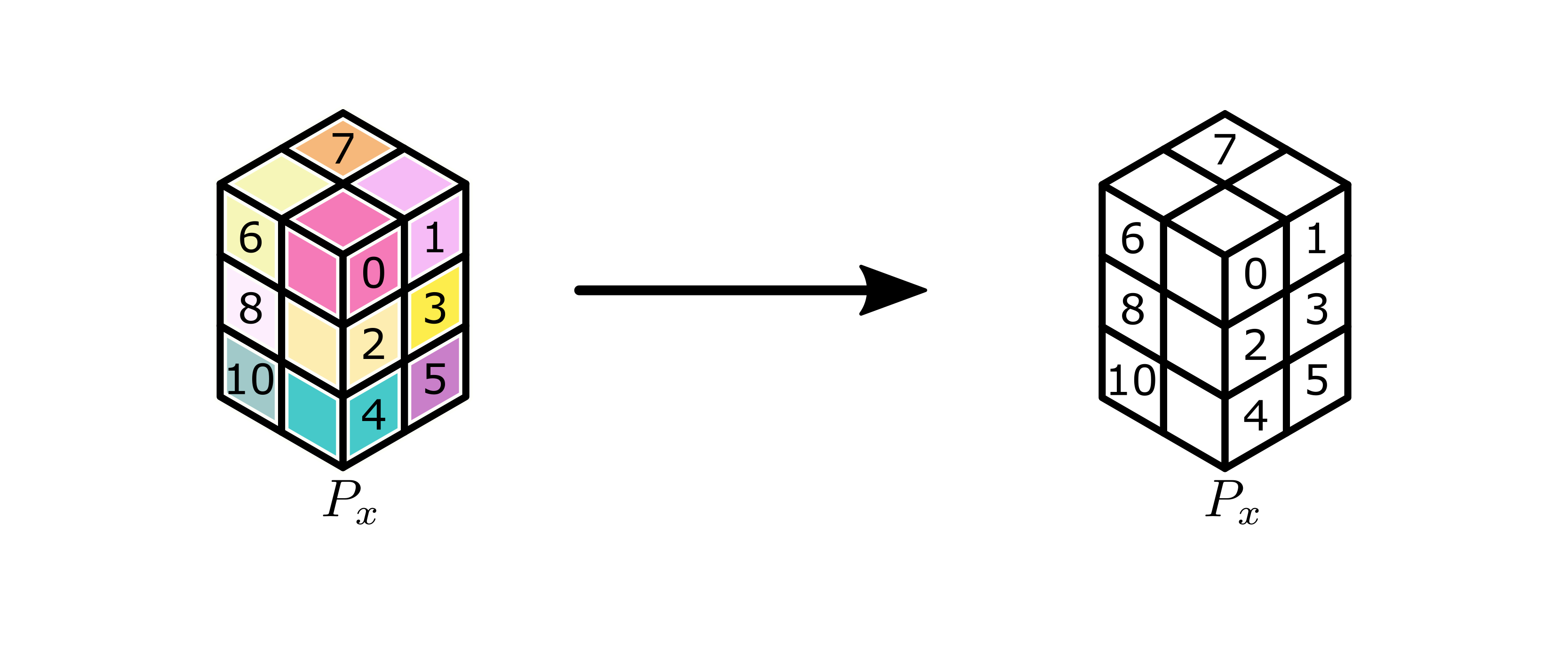
We illustrate some examples of the construction of these partitions in the following example. Consider a \(2 \times 3 \times 2\) input partition \(P_x\), as illustrated below, where workers are identified a global lexicographic ordering. For example, in an MPI-based environment, this would mean the identifiers are the ranks in a group of size 12 that is a parent group to both partitions.

Note

Implementations should not impose anything on the ordering of the workers. Back-end specific (private) routines may be used to map indices to workers.

Caption here.

If the reduction is specified over the 0th and 2nd dimensions, then this broadcast creates 3 partitions as described above, illustrated below, which we label \(P_0\), \(P_1\), and \(P_2\) for convenience.

The following table gives the global lexicographic identifiers of each worker in the partition.

Partition	Workers
\(P_0\)	0, 1, 6, 7
\(P_1\)	2, 3, 8, 9
\(P_2\)	4, 5, 10, 11

After the forward application of the all-sum-reduction, all workers active in the P_x partition have as output the sum reduction of the correct subtensors of the original tensor.

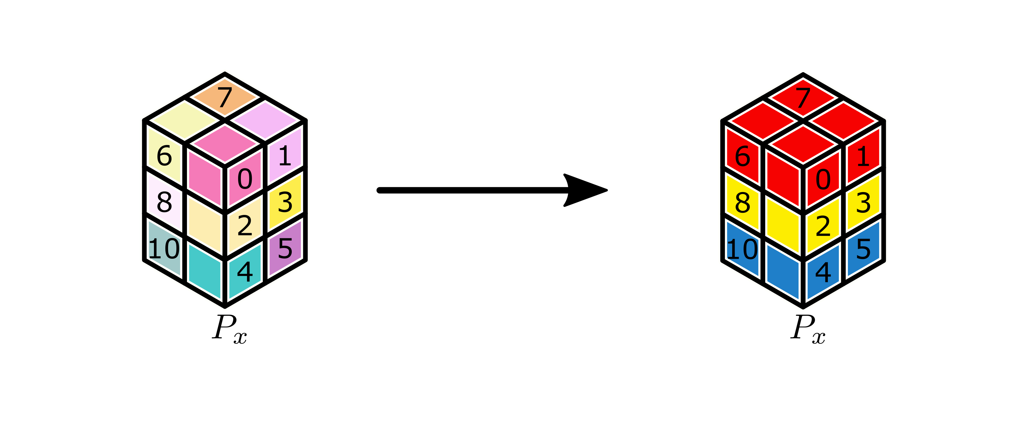
Completed all-sum-reduction.

AllSumReduce may apply over any combination of the dimensions, including all and none of them. If all dimensions of the partition are included, the output is the sum over all input tensors in the partition. If the set of input dimensions is empty, then the layer is functionally the identity.

The adjoint phase works the same way, as this operation is self-adjoint, as described in the motivating paper.

Broadcast

Back-end	Module	Class
MPI	backends.mpi.functional.broadcast	BroadcastFunction

The functional primitive for the Broadcast data movement operation does not use the original tensor partitions \(P_x\) (input) and \(P_y\) (output) directly. Instead, the calling class must create two new partitions to enable actual data movement.

For the Broadcast operation, these are back-end specific implementations of Partitions with No Topology and the data movement occurs within these partitions.

The partitions are created using the create_broadcast_partition_to() method of the Partition class for the selected back-end, which creates a number of partitions equal to the product of the shape of \(P_x\).

Each of these partitions has, as its root, the worker that is the source of the data to be copied in the broadcast and all other workers in the partition are to receive those copies. The root is specified in a back-end specific manner, e.g., the first worker in the partition is the 0th rank in the associated group of processors in the MPI back-end implementation.

Each worker in \(P_x\) or \(P_y\) has access to up to two of these partitions. If the worker is active in \(P_x\) it will have a non-null P_send partition, which it is the root worker of. If it is active in \(P_y\), it will have a non-null P_recv partition. Usually, the worker will be a non-root worker in P_recv, indicating that it is going to receive a copy from the root. However, it is possible that the worker may be the root of P_recv. This occurs if P_send and P_recv are the same and thus the worker is required to copy its own data to itself as part of the broadcast.

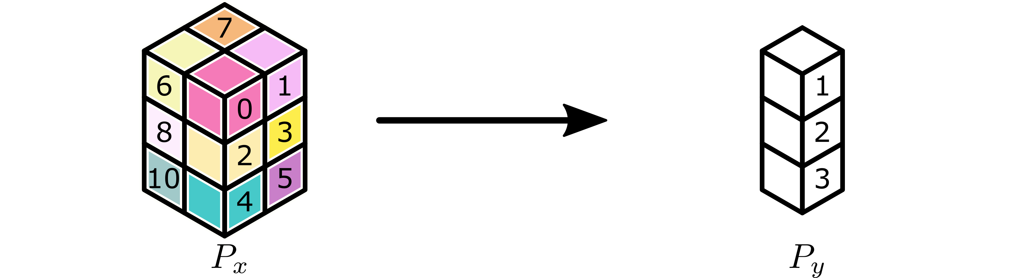
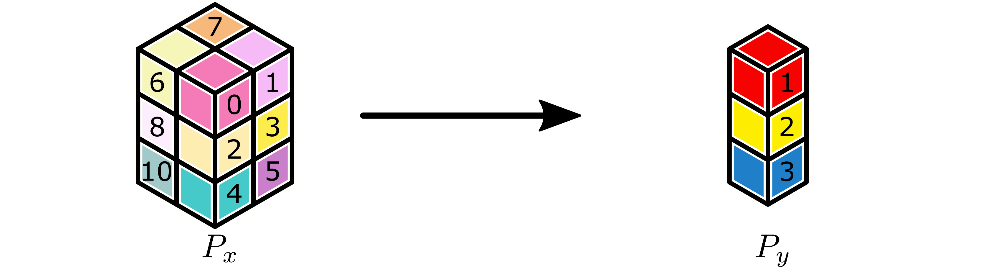
We illustrate some examples of the construction of these partitions in the following example. Consider a broadcast of a tensor partitioned by a \(1 \times 3 \times 1\) partition \(P_x\) to \(2 \times 3 \times 2\) partition \(P_y\), as illustrated below, where workers are identified a global lexicographic ordering. For example, in an MPI-based environment, this would mean the identifiers are the ranks in a group of size 12 that is a parent group to both partitions.

Note

Implementations should not impose anything on the ordering of the workers in \(P_x\) and \(P_y\). The sets of workers in these partitions may be disjoint, partially overlapping, or completely overlapping.

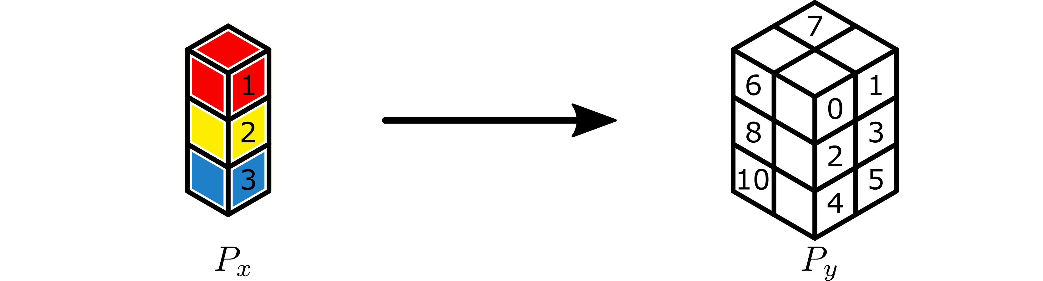
Blue, yellow, and red subtensors on \(P_x\) are to be broadcast to \(P_y\). Labels on subtensors are global lexicographic identifiers for the workers.

This broadcast creates 3 partitions as described above, illustrated below, which we label \(P_0\), \(P_1\), and \(P_2\) for convenience.

The following table gives the global lexicographic identifiers of each worker in the partition, with the root worker listed first in bold.

Partition	Workers
\(P_0\)	1, 0, 6, 7
\(P_1\)	2, 3, 8, 9
\(P_2\)	3, 4, 5, 10, 11

The following table gives the partition label for the partition that each worker associates with P_send and P_recv.

Worker	P_send	P_recv		Worker	P_send	P_recv		Worker	P_send	P_recv
0	n/a	\(P_0\)		4	n/a	\(P_2\)		8	n/a	\(P_1\)
1	\(P_0\)	\(P_0\)		5	n/a	\(P_2\)		9	n/a	\(P_1\)
2	\(P_1\)	\(P_1\)		6	n/a	\(P_0\)		10	n/a	\(P_2\)
3	\(P_2\)	\(P_1\)		7	n/a	\(P_0\)		11	n/a	\(P_2\)

This example illustrates the case where a worker needs to broadcast to itself as root (workers 1 and 2), the case where a worker broadcasts from itself as root and receives data in another partition (worker 3), and the case where a worker simply receives copies of the data from the roots (workers 0 and 4-11). It also illustrates that the root worker is the one that has the data, not the lowest globally ranked worker (e.g., in \(P_0\)).

After the forward application of the broadcast, all workers active in a P_recv partition have as output a copy of the correct subtensor of the original tensor.

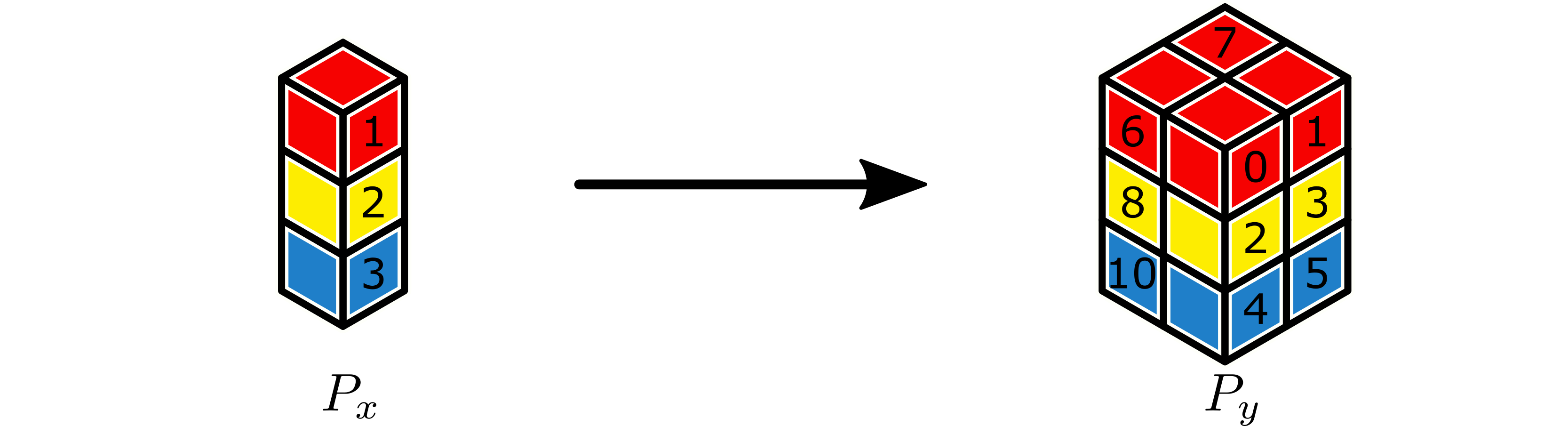
Completed broadcast.

The adjoint phase works the same way, but in reverse. However, as demonstrated in the motivating paper, the subtensors on \(P_y\) are sum-reduced back to \(P_x\), rather than copied.

Halo Exchange

Sum-Reduce

Back-end	Module	Class
MPI	backends.mpi.functional.sum_reduce	SumReduceFunction

The functional primitive for the SumReduce data movement operation does not use the original tensor partitions \(P_x\) (input) and \(P_y\) (output) directly. Instead, the calling class must create two new partitions to enable actual data movement.

For the sum-reduce operation, these are back-end specific implementations of Partitions with No Topology and the data movement occurs within these partitions.

The partitions are created using the create_reduction_partition_to() method of the Partition class for the selected back-end, which creates a number of partitions equal to the product of the shape of \(P_y\).

Each of these partitions has, as its root, the worker that is the destination of the data to be reduced in the sum-reduction and all other workers in the partition are the sources of that data. The root is specified in a back-end specific manner, e.g., the first worker in the partition is the 0th rank in the associated group of processors in the MPI back-end implementation.

Each worker in \(P_x\) or \(P_y\) has access to up to two of these partitions. If the worker is active in \(P_x\) it will have a non-null P_send partition. If it is active in \(P_y\), it will have a non-null P_recv partition, which it is the root worker of. Usually, the worker will be a non-root worker in P_send, indicating that it is going to send partial sums to the root. However, it is possible that the worker may be the root of P_recv. This occurs if P_send and P_recv are the same and thus the worker also contributes its own data to its reduction.

We illustrate some examples of the construction of these partitions in the following example. Consider a sum-reduction of a tensor partitioned by a \(2 \times 3 \times 2\) partition \(P_x\) to \(1 \times 3 \times 1\) partition \(P_y\), as illustrated below, where workers are identified a global lexicographic ordering. For example, in an MPI-based environment, this would mean the identifiers are the ranks in a group of size 12 that is a parent group to both partitions.

Note

Implementations should not impose anything on the ordering of the workers in \(P_x\) and \(P_y\). The sets of workers in these partitions may be disjoint, partially overlapping, or completely overlapping.

Colored subtensors on \(P_x\) to be sum-reduced to \(P_x\). Labels on subtensors are global lexicographic identifiers for the workers.

This broadcast creates 3 partitions as described above, illustrated below, which we label \(P_0\), \(P_1\), and \(P_2\) for convenience.

The following table gives the global lexicographic identifiers of each worker in the partition, with the root worker listed first in bold.

Partition	Workers
\(P_0\)	1, 0, 6, 7
\(P_1\)	2, 3, 8, 9
\(P_2\)	3, 4, 5, 10, 11

The following table gives the partition label for the partition that each worker associates with P_send and P_recv.

Worker	P_send	P_recv		Worker	P_send	P_recv		Worker	P_send	P_recv
0	\(P_0\)	n/a		4	\(P_2\)	n/a		8	\(P_1\)	n/a
1	\(P_0\)	\(P_0\)		5	\(P_2\)	n/a		9	\(P_1\)	n/a
2	\(P_1\)	\(P_1\)		6	\(P_0\)	n/a		10	\(P_2\)	n/a
3	\(P_1\)	\(P_2\)		7	\(P_0\)	n/a		11	\(P_2\)	n/a

This example illustrates the case where a worker needs to sum-reduce to itself as root (workers 1 and 2), the case where a worker sum-reduces from itself as root and receives data in another partition (worker 3), and the case where a worker simply contributes data to the reduction (workers 0 and 4-11). It also illustrates that the root worker is the one that has the data, not the lowest globally ranked worker (e.g., in \(P_0\)).

After the forward application of the sum-reduction, all workers active in a P_recv partition have as output the sum-reduction of the appropriate subtensors of the original tensor.

Completed sum-reduction. CMY channels of \(P_x\) subtensors add up to red, yellow, and blue subtensors of \(P_y\).

The adjoint phase works the same way, but in reverse. However, as demonstrated in the motivating paper, the subtensors on \(P_y\) are broadcast back to \(P_x\), rather than sum-reduced.

Transpose

Back-end	Module	Class
MPI	backends.mpi.functional.repartition	BroadcastFunction

The functional primitive for the Transpose data movement operation does not use the original tensor partitions \(P_x\) (input) and \(P_y\) (output) directly. Instead, the calling class creates a new union partition, within which data is moved.

Within this union, workers either share data with other workers, receive shared data from other workers, or keep subsets of their own data. All sharing of data occurs through intermediate buffers.

Note

These buffers are allocated by the calling class, using a helper function that must be specified by the back-end.

The calling class provides two sets of meta information and buffers, one for any sending and one for any receiving a worker has to do. The meta information is a triplet, (slice, size, partner). When the worker must send data, slice is a Python Slice object describing the indices of the input tensor that it must copy to worker partner. size is the volume of slice and partner is the lexicographic identifier (or rank) of the partner worker. The associated send buffer will be of size size, specified in records, not bytes. Meta information for the receive is essentially the same, except slice describes the slice of the output tensor the data will go to and partner is the source the data.

While most operations can be completed using information about the local subtensor only, this operation requires the global input tensor size. This is because we do not require the global tensor size to be specified when the layer is instantiated. Instead, the layer determines that size when it is called. Consequently, the shape of the local output subtensor tensor cannot be known until then, either.

A worker may be part of either \(P_x\), \(P_y\), or both. If it is part of \(P_x\), then it will only need to share parts of its local input subtensor with other workers. If it is not part of \(P_x\), it will take a zero-volume tensor as input. If it is part of \(P_y\), its output subtensor will be formed by receiving copies of parts of other workers’ local input subtensors. If it is not part of \(P_y\), then its output will be a zero-volume tensor. If a worker is part of both, its output may be a direct copy of part of its own input.

The adjoint phase works the same way, but in reverse. However, as demonstrated in the motivating paper, the subtensors on \(P_y\) are summed back to \(P_x\), rather than copied. However, because there are no overlaps in the local scatters, this sum can safely be replaced with a copy.

Backends

MPI Backend

The MPI data movement backend.