Repartition Layer
Overview
The Repartition distributed data movement primitive performs a repartition, shuffle, or generalized all-to-all operation of a tensor from one partition to another.
In DistDL, the Repartition allows you to change how tensor data is distributed across workers, which allows for more optimal communication patterns and load balancing.
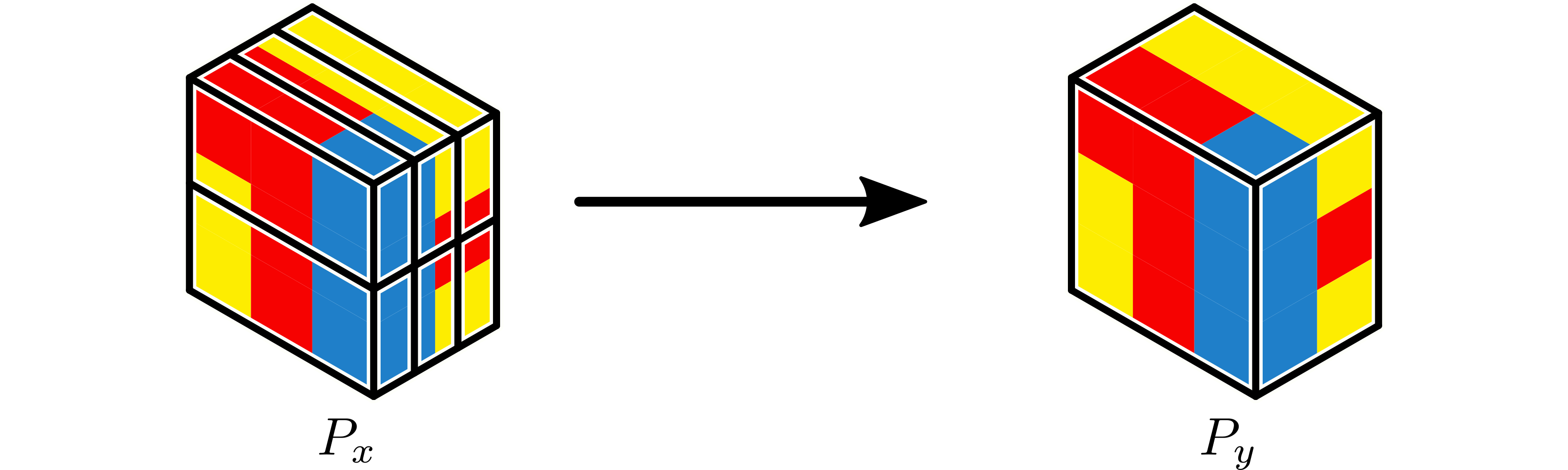
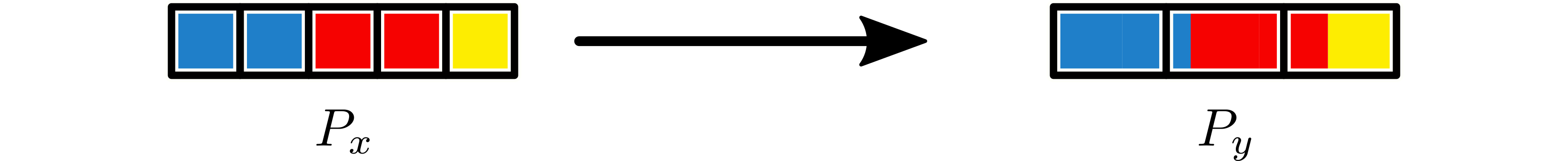
For the purposes of this documentation, we will assume that an arbitrary global input tensor \({x}\) is partitioned by \(P_x\) and that another partition \(P_y\) exists.
Note
The repartition operation in DistDL has similar flavor to the classical
parallel all-to-all operation. However, DistDL focuses on exploiting
structure on the data, while the classical all-to-all usually assumes 1D
(or quasi-1D) data (e.g., in the sense of MPI_Alltoall()).
Motivation
In distributed deep learning, consecutive layers have potentially widely varying structure. It is very common to see changes in the number of degrees of freedom in the feature dimensions, the number of channels, and even the number of dimensions in the tensors themselves.
Parallel load balance is driven by data layout and kernel structure, so given this variability, the parallel data distribution of the output of one layer may not be the optimal distribution for the input of the next.
The Repartition layer provides a mechanism to change the data distribution, that is to change the partition partition function on a tensor, as needed.
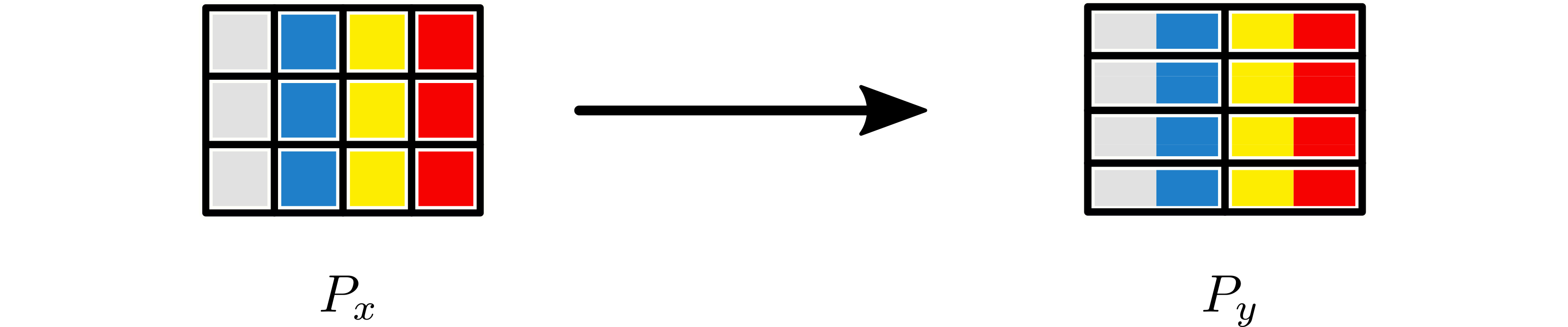
This primitive draws its inspiration from the parallel all-to-all pattern, which has the appearance of transposing a matrix, from a certain perspective.
For example, consider a 16-length array, distributed over 4 workers.

This array can be viewed as a \(4 \times 4\) matrix, partitioned in a row contiguous way.
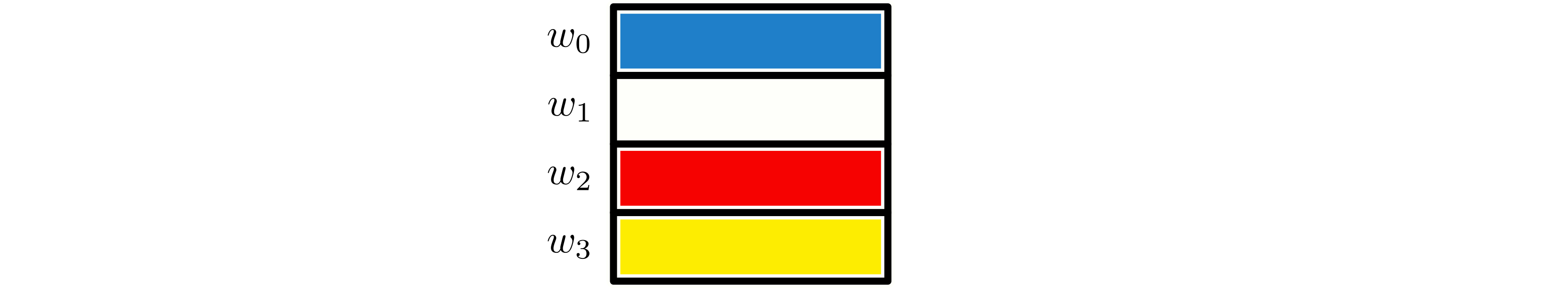
The all-to-all pattern remaps the array as if the \(4 \times 4\) matrix has been repartitioned, so the column-contiguous view becomes row contiguous.
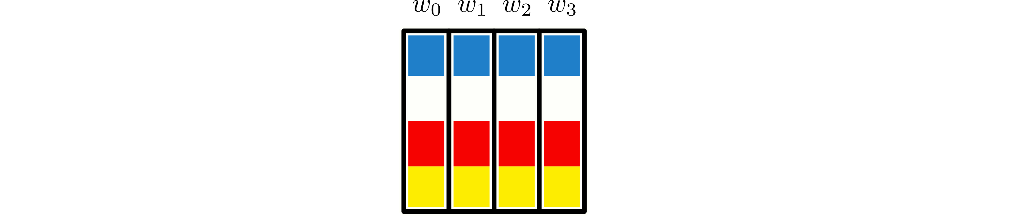
Thus, the new view distribution of the data is as follows.

Implementation
A back-end functional implementation supporting DistDL
Repartition must complete the repartition operation, as
described below.
Consider two partitions of the same tensor. The Repartition operation performs the necessary data movements such that the tensor, stored on the first partition, can be remapped to the second partition.
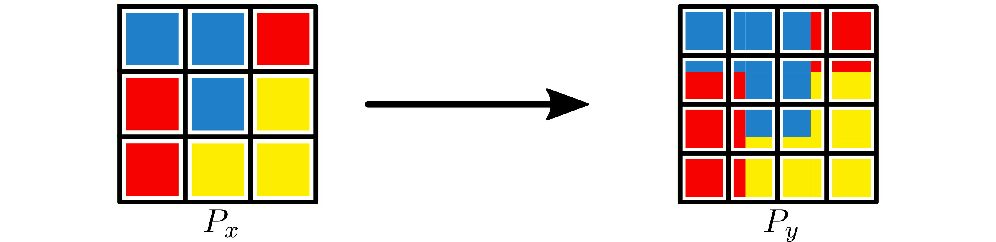
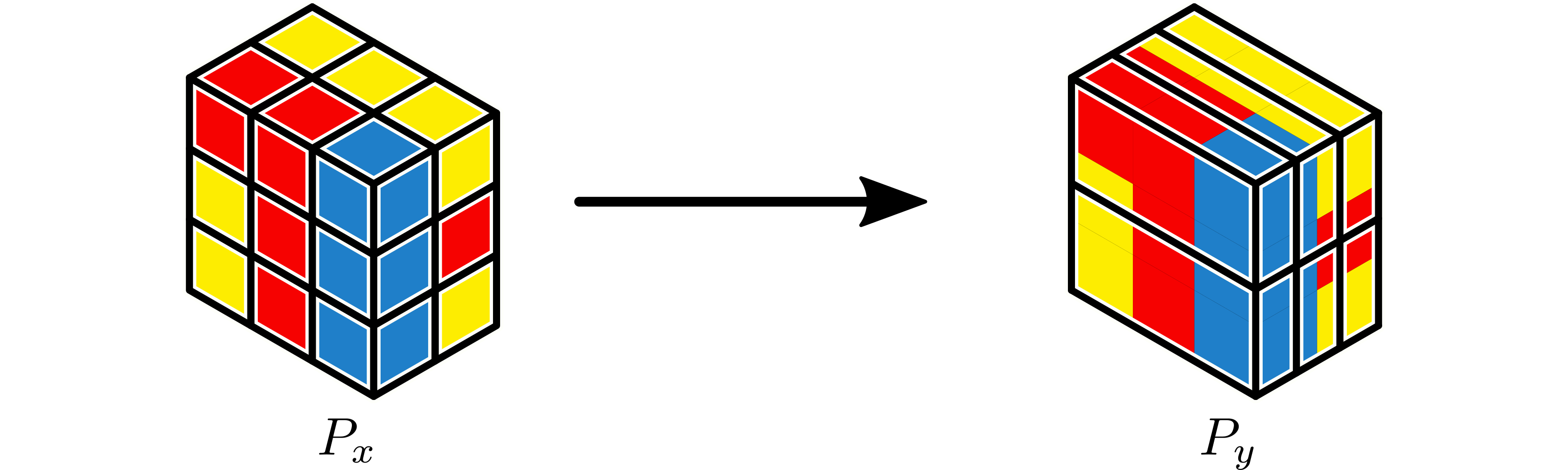
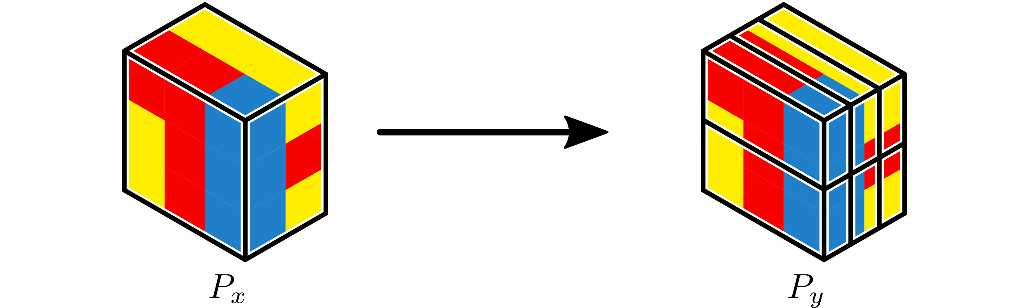
Example Repartition from \(P_x\), a \(3 \times 3\) partition, to \(P_y\), a \(4 \times 4\) partition.
The data movement in a Repartition operation is inherently dependent on the overlap between a subtensor in \(P_x\) and all subtensors in \(P_y\). In sketching the behavior, we will examine the behavior of the middle subtensor/worker in \(P_x\) pt 1.
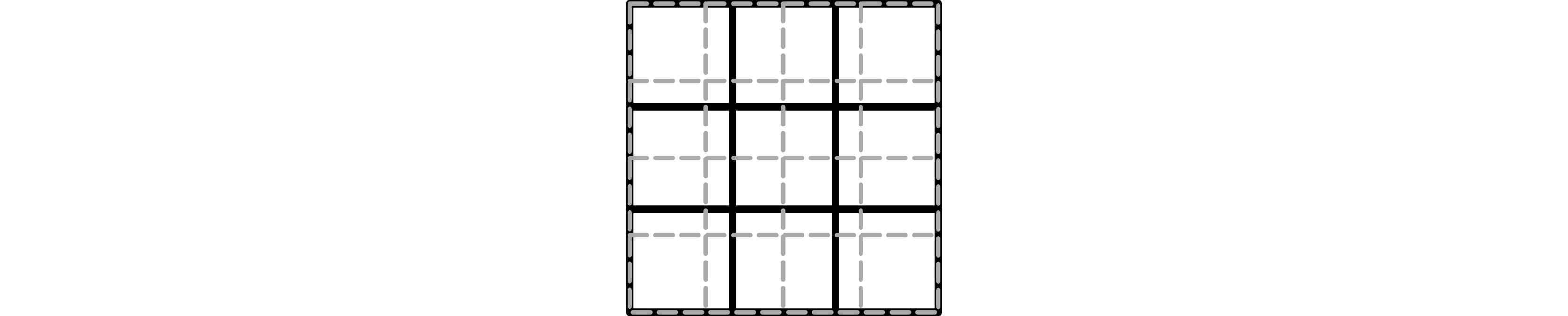
Overlap of a \(3 \times 3\) partition (black) and a \(4 \times 4\) partition (grey).
Assumptions
The dimension of \(P_x\) matches the dimension of \(x\).
The dimension of \(P_y\) matches the dimension of \(x\).
Consequently, the dimension of both partitions needs to be the same.
Note
These requirements may require a new partition to be created. As long as the essential structure of the partition is preserved (total number of workers, mapping of tensor dimensions to workers, etc.) then new partitions can be created with arbitrary dimensions of length 1 can be created. For example, a \(3\) partition can become \(1 \times 1 \times 3\) without a repartition, and the new partition can be used as an input to the repartition.
Input tensors do not have to be load-balanced. Output tensors will always be load balanced.
Note
Consequently, if an input tensor is unbalanced on a partition, a repartition to the same partition will rebalance it.
Intermediate data movement may be required by an implementation. This may require intermediate buffers. Buffer management should be a function of the back-end, as different communication back-ends may require different structure for buffers.
Warning
The current implementation has buffer allocation directly in the primal interface class. This will be resolved in the future.
Forward
The forward implementation of repartition maps a tensor from one Cartesian partition to another, without changing the partition. From the perspective of one worker in \(P_x\), this operation looks like a multi-dimensional scatter.
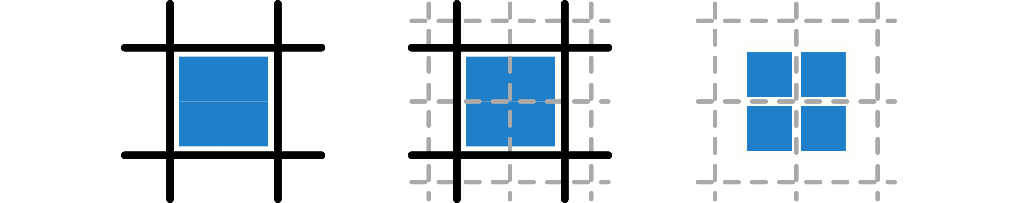
Left: Data on current (middle) worker of \(P_x\). Middle: Overlapping partition boundaries. Right: Data from current worker on 4 middle workers of \(P_y\).
The setup is determined by the sequence of overlaps of the subtensor owned by
the current worker and the subtensors owned by the workers in \(P_y\). The
amount of overlap is different from pair to pair, so the volume of data
movement is also different. Thus, from the perspective of one worker in
\(P_x\), this is like a multi-dimensional MPI_Scatterv.
Adjoint
The adjoint implementation of repartition also maps a tensor from one Cartesian partition to another, without changing the partition. From the perspective of one worker in \(P_x\), this operation looks like a multi-dimensional gather.
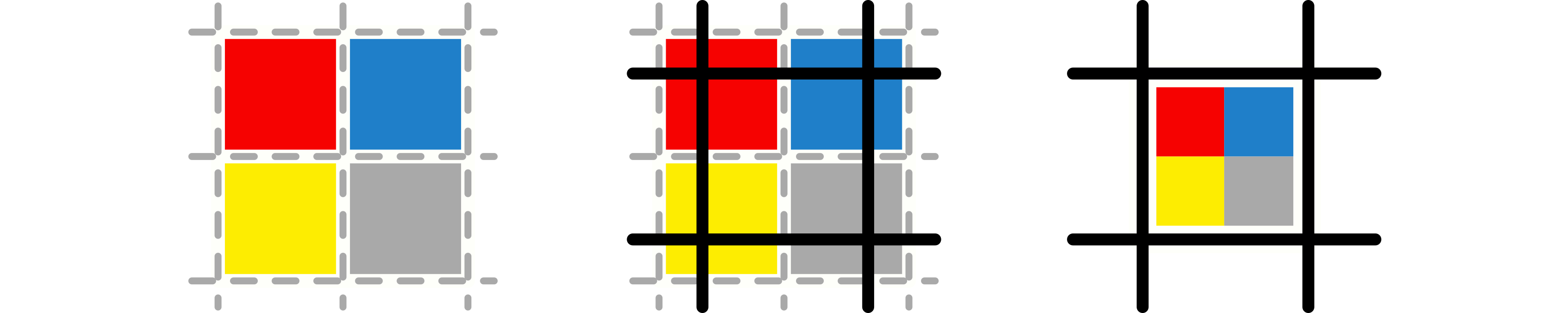
Left: Data on 4 middle workers of \(P_y\) partition. Middle: Overlapping partition boundaries. Right: Data from 4 middle workers of \(P_y\) copied back to current (middle) worker of \(P_x\).
The setup is determined by the same sequence of overlaps as the forward
operation. Thus, from the perspective of one worker in \(P_x\), this is
like a multi-dimensional MPI_Gatherv.
Examples
Use Cases
Example 1: Remap 1D Partition
If \(x\) is a 1D tensor, a partition with shape \(5\), can be repartitioned to a partition with shape \(3\).
Example 2: Remap 2D Partition
If \(x\) is a 2D tensor, a partition with shape \(3 \times 4\), can be repartitioned to a partition with shape \(4 \times 2\).
Example 3: Remap 3D Partition
If \(x\) is a 3D tensor, a partition with shape \(3 \times 2 \times 2\), can be repartitioned to a partition with shape \(1 \times 2 \times 3\).
Example 4: Repartition as Scatter
Repartition can be used to scatter tensors. For example, if one worker reads data from disk, repartition can be used to scatter it to a number of workers. If there is a partition of dimension 1 containing a tensor \(x\) of dimension 3, by extending the input partition to \(1 \times 1 \times 1\) it can be repartitioned to a partition of dimension \(1 \times 3 \times 2\).
Example 5: Repartition as Gather
Repartition can be used to gather tensors. For example, if one worker outputs data to disk, repartition can be used to gather it from a number of workers. If there is a partition of dimension \(1 \times 3 \times 2\) containing a tensor \(x\) of dimension 3, it can be mapped to a partition of dimension \(1\) by extending the output partition to \(1 \times 1 \times 1\) and applying a repartition.